Parameter Updating

Context

A Bayesian network compactly represents the Joint Probability Distribution of a domain that is defined by variables.
Both the qualitative and quantitative parts of a Bayesian network are based on analyzing observations or "particles" sampled from this domain.
- If experts design a Bayesian network manually, pieces of expert knowledge can be considered particles.
- If a Bayesian network is machine-learned, each record in the dataset associated with the network is a particle.

Qualitative Part

Creating the qualitative part of a Bayesian network consists of adding arcs between nodes for representing their direct probabilistic relationships.
- In the context of expert-based modeling, arcs can be defined in brainstorming sessions, by a group of experts, for instance.
- In the context of machine learning, the particles in a dataset are analyzed to discover probabilistic relationships between variables automatically.

Quantitative Part

Generating the quantitative part of a Bayesian network consists of specifying the probability distributions associated with each node.
- In BayesiaLab, the probability distributions of nodes are represented by default with tables.
- For Root Nodes, which are nodes that do not have any incoming arcs, a simple Probability Table with one probability value per state can represent the marginal distribution.
- For nodes that do have Parent Nodes, we require a Conditional Probability Table, i.e., one probability value for each combination of the Parent Nodes' states to represent the distribution.
- For illustration only, we have this simple network consisting of the Parent Node, Eye Color, and the Child Node, Hair Color, which are connected by an arc.
- The Parent Node features a Probability Table.
- The Child Node features a Conditional Probability Table.
In the context of expert-based modeling, these probabilities can be estimated in brainstorming sessions using BEKEE.
In the context of machine learning, BayesiaLab estimates the probabilities using the Maximum Likelihood Estimation method, which means that the probability of each state corresponds to its observed frequency in the dataset.
- Hence, this method is purely frequentist.
- However, it is possible to introduce a Bayesian approach with this methodology by mixing the observed particles from the dataset with virtual particles defined by Dirichlet Priors.

Dirichlet Priors

Even though the focus of this page is Parameter Updating, we need to provide context by referencing two other functions that can define Dirichlet priors, i.e., [Generate Prior Samples](/Users/stefanconrady/Library/CloudStorage/OneDrive-BayesiaUSA/ClickHelp Backup/project-backup_bayesialab_2024-06-07_08-24-26/HTML/data-prior-samples-generate.html) and [Edit Number of Uniform Prior Samples](/Users/stefanconrady/Library/CloudStorage/OneDrive-BayesiaUSA/ClickHelp Backup/project-backup_bayesialab_2024-06-07_08-24-26/HTML/edit-edit-number-of-uniform-prior-samples.html).

Generate Prior Samples

[Generate Prior Samples](/Users/stefanconrady/Library/CloudStorage/OneDrive-BayesiaUSA/ClickHelp Backup/project-backup_bayesialab_2024-06-07_08-24-26/HTML/data-prior-samples-generate.html) creates virtual particles (or prior samples) according to the Joint Probability Distribution represented by the current Bayesian network.

Edit Number of Uniform Prior Samples

Uniform Prior Samples are a way to specify a specific kind of prior knowledge, namely the belief that all nodes are marginally independent, which would be the equivalent of a fully unconnected network.
For instance, setting Uniform Prior Samples to 1, means that one virtual particle (or virtual observation/occurrence) would be "spread across" all states of all nodes, assigning a fraction of this virtual particle to all cells.
As a result, the network stipulates that "nothing is impossible."
As these virtual particles are mixed with those described in the data set, Dirichlet priors not only impact the estimation of the probabilities but also bias the structural search.

Parameter Updating

The third way of defining Dirichlet Priors is Parameter Updating.
Parameter Updating uses the observations/evidence you set via the Monitors as particles for updating the quantitative part of the current Bayesian network.
So, these particles update the probability distributions of the corresponding observed nodes plus the probability distributions of their unobserved ancestors.
This implies that such particles do not have to be completely observed in all the dimensions that are represented by the Bayesian network. For instance, a network may consist of ten nodes, N1 through N10, but the particle that updates this network consists only of one observation, e.g., N8=True, with all other nodes remaining unobserved.
The Joint Probability Distribution encoded by the current Bayesian network defines the Dirichlet Priors.
As new particles are observed via the Monitors and get mixed with the virtual particles of the prior, a weighting is required, the so-called Prior Weight.
The Prior Weight specifies the relative importance of the prior by assigning an equivalent number of virtual particles.
As a result, a Prior Weight of 1 would mean that the prior Joint Probability Distribution would quickly be "overruled" by a few new observations via the Monitors.
A Prior Weight of 1,000,000, however, would take a large number of new observations to materially affect the prior Joint Probability Distribution.
Additionally, you can use a Discount factor to "fade out" the importance of the prior Joint Probability Distribution as new particles are observed. This gradually reduces the number of virtual particles from the prior Joint Probability Distribution and, thus, its weight relative to the new particles.

Usage

To start Parameter Updating with a given Bayesian network, select Menu > Inference > Parameter Updating.
To illustrate the use of Parameter Updating, we present two examples, the first one with a single node, and the second one with two nodes.

Examples

Types of Evidence

All the BayesiaLab types of evidence can be used to describe the particles:

Hard Positive Evidence: no uncertainty on the state of the variable, i.e. all the likelihoods of the other states are set to 0%;
Hard Negative Evidence: the likelihood of one state is set to 0% while the other ones are set to 100%;
Likelihood Evidence: a likelihood distribution is associated with the node. To be informative, the distribution should contain at least one likelihood that differs from the other ones;
Probabilistic Evidence: a likelihood distribution is computed for getting the required probability distribution. It's possible to define a static likelihood distribution ( computed just once, when the evidence is set), or a dynamic likelihood distribution ( updated after each new piece of evidence for maintaining constant the required probability distribution).
Numerical Evidence: a probability distribution is estimated to get the required expected value (with the MinXEnt (opens in a new tab), Binary (opens in a new tab), or Shift (opens in a new tab) estimation methods). A likelihood distribution is then computed for getting the computed probability distribution. It's possible to define a static likelihood distribution (computed just once, when the evidence is set), or a dynamic likelihood distribution ( updated after each new piece of evidence for maintaining constant the required probability distribution or required expected value).

Source of Observations

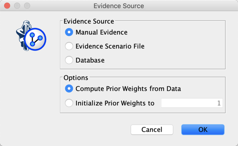
There are three evidence sources for describing the particles:

Manual Evidence: utilization of the monitors in the Monitor Panel, or the new interactive rendering of the nodes ([Monitors](/Users/stefanconrady/Library/CloudStorage/OneDrive-BayesiaUSA/ClickHelp Backup/project-backupbayesialab_2024-06-07_08-24-26/HTML/35651944.html#RenderingProperties(8.0)-Monitor1337599028), [Gauges](/Users/stefanconrady/Library/CloudStorage/OneDrive-BayesiaUSA/ClickHelp Backup/project-backup_bayesialab_2024-06-07_08-24-26/HTML/35651944.html#RenderingProperties(8.0)-Gauge1337599028) or [Bars](/Users/stefanconrady/Library/CloudStorage/OneDrive-BayesiaUSA/ClickHelp Backup/project-backup_bayesialab_2024-06-07_08-24-26/HTML/35651944.html#RenderingProperties(8.0)-Bar1337599028)) in the **_Graph Panel**; All types of evidence can be used;
Evidence Scenario File: the scenarios can use all types of evidence;
Database: the observations are only based on Hard Positive Evidence.

When the selected evidence source is an Evidence Scenario File or the associated dataset, two additional tools are added in the toolbar compared to the manual mode: :

: carries out the update by using all the particles contained in the evidence source sequentially;
: carries out the update by using all the particles contained in the evidence source in batch, until the entropy of the observations converges. Note that it comes back to the particle that was described when the process has been triggered.

While the text field is passive in the Manual Mode (i.e., it indicates how many particles have been taken into account for updating the tables), it can be utilized in the other two modes to indicate the index of the last particle to be processed.

Smoothed Probability Estimation

The option available via Menu > Edit > Edit Smoothed Probability Estimation allows generating particles from the uniform joint distribution. Interestingly, the exact same result can be achieved by setting uniform distribution in all the tables of the network (marginal and conditional) and then using the Database Source for updating the parameters.

Example

Suppose we have the network below and an associated dataset containing 100 records or observations.

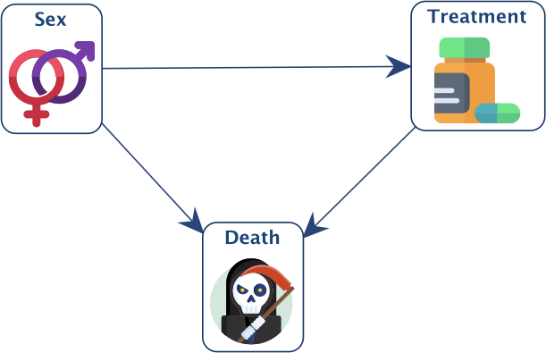
In order to implement the Smoothed Probability Distribution, we first set the three tables to uniform distributions:

We set Discount to its default value 1, then select Database as the Evidence Source**,** and set our Prior Weight to 1.

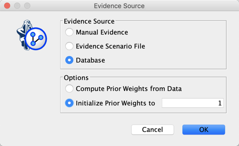
Upon clicking ![/images/35652368.png], all the particles described in the data set are utilized for updating the probability distributions.

saves the updated tables, which are exactly identical to those you would get using [Smoothed Probability Estimation](/Users/stefanconrady/Library/CloudStorage/OneDrive-BayesiaUSA/ClickHelp Backup/project-backup_bayesialab_2024-06-07_08-24-26/HTML/2851198.html).

Evidence Instantiation

[Evidence Instantiation](/Users/stefanconrady/Library/CloudStorage/OneDrive-BayesiaUSA/ClickHelp Backup/project-backup_bayesialab_2024-06-07_08-24-26/HTML/2851246.html), introduced in version 5.0.4, creates a network based on the current network and a set of evidence. While the original network and the evidence define a subspace in the original joint probability distribution, the new instantiated network is entirely dedicated to the representation of that subspace. This is very useful in at least two scenarios:

You want to set evidence on a subset of nodes, while keeping these nodes in the set of “drivers” (e.g. Target Optimization) or analyzed nodes (e.g. [Target Analysis]),
You have designed your network (usually by using expert knowledge), and some marginalized distributions do not exactly match knowledge you have about marginal distributions. So you want to automatically adjust the conditional probability distributions to get these marginal distributions.

In the case of evidence set on a common child of two marginally independent nodes, the exact instantiation was not possible because of the conditional dependency.

It is now possible to use Parameter Updating to obtain a much better instantiation for all set of evidence.

Example

Suppose we have the network below

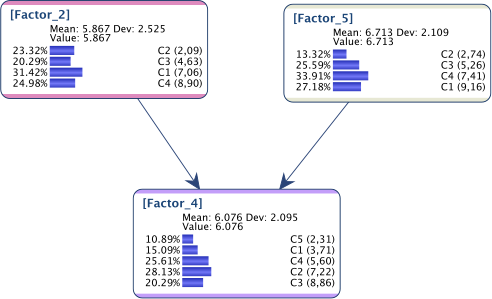
and for some reason, we want to get the following marginal distributions, set with Fixed Numerical Evidence:

[Evidence Instantiation]
[Parameter Updating]

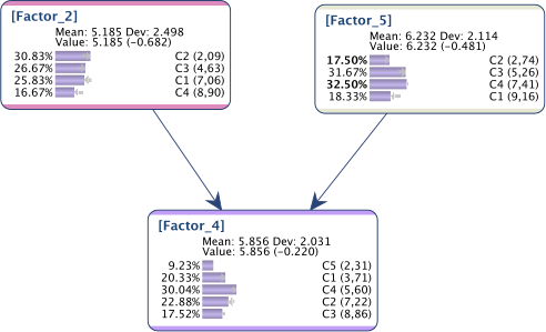
Below is the instantiated network obtained with Evidence Instantiation:

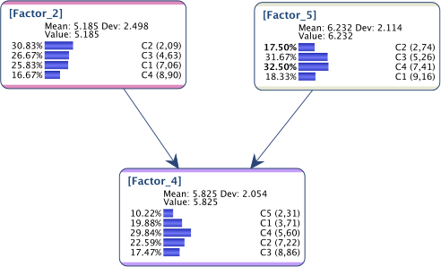
As we can see, whereas the distributions are correct for Factor_2 and Factor_5, it's not the requested one for the collider Factor_4.

We first need to store this set of numerical evidence in the scenario file .

We then set a Discount of 0 for all the nodes so as not to mix our particle with any prior. We then select Evidence Scenario File as as source of evidence. Note that Prior Weight does not matter because Discount is zero.

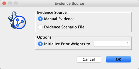
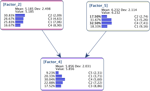
Clicking on ![/images/35652369.png] allows using these three pieces of evidence until the entropy of the observations converges.

As we can see below, the updated model perfectly represent the requested marginal distributions.

Expectation-Maximization

When the data set contains missing values, or when the network has hidden nodes (i.e. with 100% missing values), the estimation of the probabilities is done by using an Expectation-Maximization (EM) algorithm. It basically consists in iterating though the following two steps until convergence:

Expectation: utilization of the current Bayesian network for completing the not fully observed particles;
Maximization: utilization of the Maximum Likelihood Estimation algorithm for updating the probabilities with the completed particles.

The Learning | Parameter Estimation method is used by all BayesiaLab machine learning algorithms, and as such, it is entirely data driven, i.e. it does not take into account the probability distributions that have been defined manually.

As of version 8.0, you can use Parameter Updating when you want EM to take your priors into account when estimating the probabilities of your network.

Example

Suppose we have the network below for which we have data for all nodes, except for Hidden Cause.

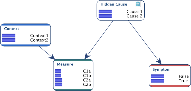
The only expert knowledge we have is expressed in the conditional distribution of Measure below. The "a" measures can only come from Context1, whereas the "b" measures can only come from Context2.

Without any expert knowledge on the other nodes, we set uniform distributions for all the other nodes.

We then set a Discount of 0 for all nodes to use only the particles described in the data set for estimating the probabilities. We then select Database as source of evidence. Note that Prior Weight does not matter because Discount is zero.

Clicking on ![/images/35652369.png] allows using all the particles described in the data set for updating the probabilities, until the entropy of the observations converges.

We get the following updated network.

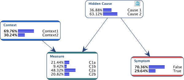
As we can see below, the prior knowledge has been taken into account during the update of the probability tables.

Hyperparameter Updating Example One Node