Structural Coefficient Analysis

Context

• When machine-learning a Bayesian network model from data, trading off the fit of the model versus the complexity of the model is one of the main tasks for the researcher.
• BayesiaLab uses the so-called Structural Coefficient as the main parameter that you can use to bias the learning algorithms in favor of better fit or less complexity.
• In a typical model development workflow, you should compare and evaluate the Bayesian network structures that were machine-learned with a range of Structural Coefficient values.
• Such a comparison allows you to judge the robustness of arcs in the network. Arcs that are discovered frequently across a wide range of Structural Coefficient values are more robust than those that are found rarely.
• Of special concern is the risk of overfitting the model to the given dataset.​ Overfitting, of course, would defeat the purpose of the model, as it can no longer generalize beyond the learning sample.
• While you could modify the Structural Coefficient manually and then run a learning algorithm for each of the values you wish to try, the Structural Coefficient Analysis performs this process automatically.

Usage

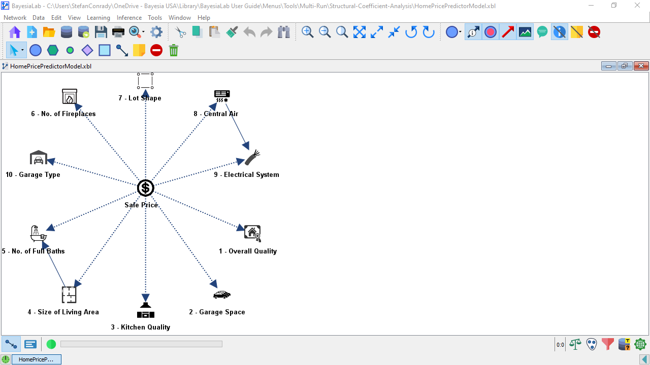
The example is derived from the Ames dataset, which represents residential real estate transactions in the city of Ames, Iowa. For more background on this dataset, please see Chapter 5: Bayesian Networks and Data. Our starting point for illustrating the Structural Coefficient Analysis workflow is a home price prediction model based on the Ames dataset. The corresponding Bayesian network model is available for download here:

HomePricePredictorModel.xbl

• Open HomePricePredictorModel.xbl in BayesiaLab.
• Note that the dataset associated with this model is split into a Learning Set and a Test Set, as indicated by the  symbol on top of the database icon  in the lower right-hand corner of the Graph Window.
• The current network, from which the following Structural Coefficient Analysis is launched, will serve as the Reference Structure.
• This Reference Structure will subsequently be compared to the newly learned Comparison Structures, i.e., the structures generated in the course of the Structural Coefficient Analysis.
  
• To start, select Main Menu > Tools > Multi-Run > Structural Coefficient Analysis.
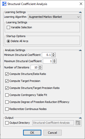
• A new window opens up that offers you a wide range of options:
  
• In this window, the options are grouped into three sections:
  • Learning Settings
  • Analysis Settings
  • Output

Learning Settings

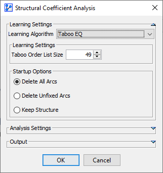
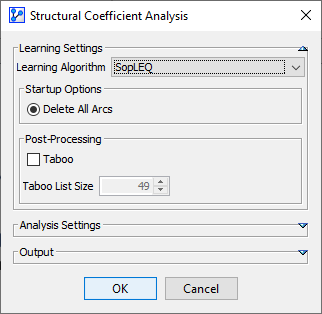
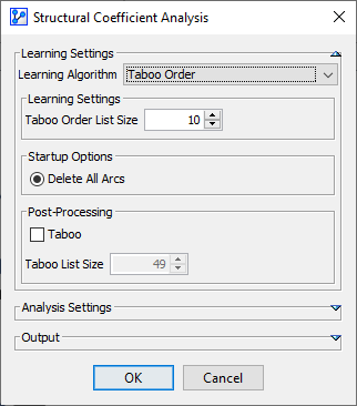
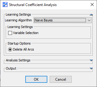
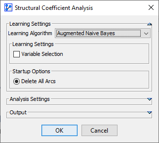
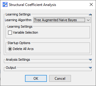
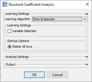
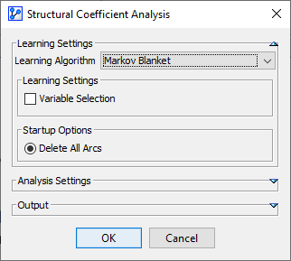
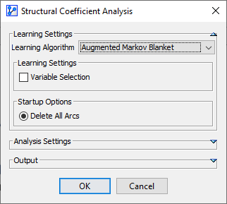
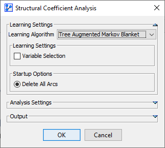
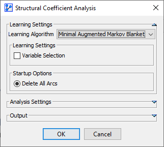
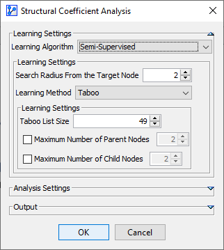
• The first option Learning Algorithm relates to the algorithm for which you want to examine different values of the Structural Coefficient. All of BayesiaLab's learning algorithms are available in this context.
• Depending on the selected algorithm, different Learning Settings and Startup Options are shown. These settings are the same that would be available if you started these learning algorithms via Main Menu > Learning.
• Click on the thumbnails in the table below to see the Learning Settings corresponding to each learning algorithm.

Taboo	EQ	Taboo EQ	SopLEQ	Taboo Order
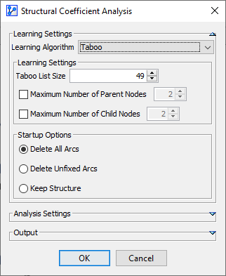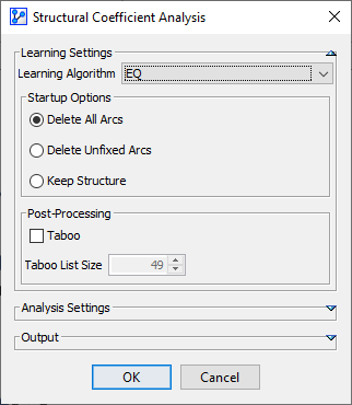Naive Bayes	Augmented Naive Bayes	Tree Augmented Naive Bayes	Sons & Spouses	Markov Blanket
Augmented Markov Blanket	Tree Augmented Markov Blanket	Minimal Augmented Markov Blanket	Semi-Supervised	Data Perturbation
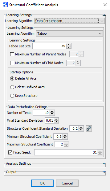Structural Priors	Partial Ordering

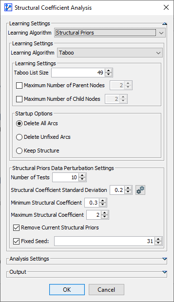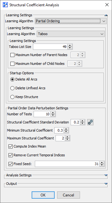Analysis Settings

• In all of the above screenshots, the Analysis Settings section and the Output section were collapsed, given that they are the same for all the learning algorithms.
• You can click on the small triangle icons to collapse or expand individual sections in this window.
• Now, we collapse the Learning Settings section and the Output section to focus exclusively on Analysis Settings.
  

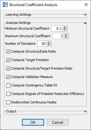
Minimum and Maximum Structural Coefficient

• The Minimum and Maximum define the range of the Structural Coefficient to be used for learning the Comparison Structures.
• The first and last Structural Coefficient values to be evaluated are the minimum and maximum of the range respectively.

Number of Iterations

• The Number of Iterations determines the number of equidistant steps between the Minimum and Maximum Structural Coefficient.
• Starting with the Minimum Structural Coefficient and using the specified learning algorithm, BayesiaLab learns a network.
• Upon completion of the network learning, the next value for the Structural Coefficient is used to learning another network.
• This repeats until the final network is learned with the Maximum Structural Coefficient.
• Here is a numerical example:
  • Minimum SC=0.1
  • Maximum SC=2
  • Number of Iterations=20
  • Therefore, the Structural Coefficient Analysis will learn a network with each of these values of the Structural Coefficient, i.e., , thus producing 20 networks.
  • Also, some of these 20 networks may be identical, i.e., two or more different Structural Coefficients may produce an identical network. As a result, you may obtain fewer Comparison Structures than the Number of Iterations you specified.

Analysis Settings — Checkboxes

• The next section within Analysis Settings contains 7 checkboxes.
  
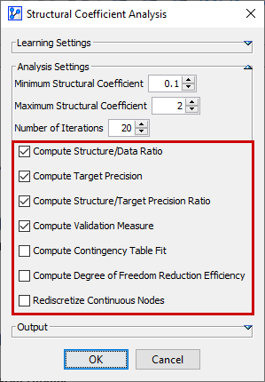
• Here, you can select the measures to be computed at each iteration, i.e., for each network.
• However, these measures are not immediately shown in the Confidence Analysis Report.
• Their purpose will become apparent once they are plotted as curves.
• From the Confidence Analysis Report you can open the Curve window and then display the measures you selected here.
• Given that the measures are meant to be interpreted visually, we defer a detailed discussion to a section dedicated to the Curve window.

Rediscretize Continuous Nodes

• Rediscretize Continuous Nodes is an option that applies to the Structural Coefficient Analysis as a whole.
• Please see the separate chapter on Rediscretize Continuous Nodes to learn about the relevance and the implications of setting this option.

Output

• The final section in the Structural Coefficient Analysis window relates to the optional output location.
  
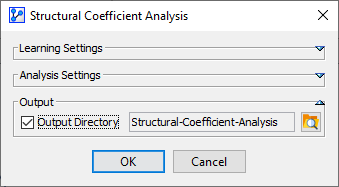
• Given that the Structural Coefficient Analysis produces multiple Comparison Structures, you specify a location to save them.
• Otherwise, you will later have an opportunity to save or extract individual Comparison Structures from the Report and the Structure Comparison.

Starting the Analysis

• Clicking OK starts the analysis.

• The Progress Bar within the Status Bar gives you a sense of how the analysis advances. Depending on the parameters you defined, this process can take a considerable amount of time.

  

• Once the analysis concludes, the Confidence Analysis Report automatically opens up in a new window.

• The Confidence Analysis Report contains a wide range of measures plus additional evaluation tools, which need to be considered jointly for determining an appropriate Structural Coefficient.

• So, please review the entire range elements of the Structural Coefficient Analysis and avoid relying on a single measure or plot:

• Confidence Analysis Report

• Curve

• Rediscretize Continuous Nodes

• Structure Comparison

• Extract Network