Missing Values Analysis

Context

• Missing values are encountered in virtually all real-world data collection processes.

• Missing values can be the result of non-responses in surveys, poor record-keeping, server outages, attrition in longitudinal surveys, or faulty sensors of a measuring device, etc.

• Missing Values Processing is an important element in machine-learning Bayesian networks. For an introduction to this topic, please see the Types of Missingness overview below and Chapter 9: Missing Values Processing in our E-Book.

• With the Missing Values Analysis function, we can see how a Bayesian network structure can affect the estimation of the missing values and, thus, changes the marginal distribution of the nodes.

• Seeing the difference in the distributions illustrates the relevance of Missing Values Processing in your current network.

• For a missing values estimation given a completely unconnected network, the distribution of missing value estimates is identical to the marginal distribution of the node's states.

  • This reflects the missing value estimates immediately upon completing the Data Import Wizard given that the Infer option was checked in Step 3 — Data Selection, Filtering, and Missing Value Processing.

• For a missing values estimation given the current network, assuming it was entirely machine-learned from data or that Parameter Estimation was performed on the most current network structure.

  • The network-based estimation produces missing value estimates that are based on the network, i.e., the estimation leverages the relationships with other nodes for estimating the distribution of the missing values.

Types of Missingness

• The Bayesian network below represents a domain in which four variables can be observed, shown in the bottom box in blue. These nodes represent the variables recorded in the dataset.

• However, the blue variables are not the actual variables of interest.
• Rather, the blue variables are merely the manifestations of the white variables in the top box, which are hidden. They contain the data of interest.
• However, with the exception of , the blue variables are not perfect replicas of the white variables.
• Instead, there is a mechanism in play, represented by a set of binary variables inside the box in the middle (red). These red nodes represent the Missingness Mechanism.
• The mechanism works as follows:
  • If a red variable is set to True, the associated blue variable is set to Missing.
  • If a red variable is set to False, the associated blue variable takes on the value of the original white variable at the top.
• Note that the mechanism itself is not observable. Like the Data-Generating Process in the top box, the Missingness Mechanism is hidden, too.
• The nodes in the red box represent three different types of missingness, which are all commonly encountered in research:
  • Missing Completely at Random (MCAR): The missingness mechanism is entirely independent of all other variables (see MCARX1). This is the ideal case as there is no bias.
  • Missing at Random (MAR): The missingness depends on observed variables (see MCARX2). By virtue of learning a network, we can capture the characteristics of this missingness mechanism and remove the bias it would otherwise introduce.
  • Missing Not at Random (MNAR): The missingness depends on hidden causes, i.e., unobserved variables, such as the data-generating variable itself (see MCARX4). This is the worst-case scenario. Given that the missingness is determined by a hidden cause, there is no way to model the mechanism, nor remove bias introduced by the missingness.

Missing Values Processing

Usage & Example

• You can start the Missing Values Analysis whenever you have a network that contains missing values.

• This tool is illustrated with a network generated by performing Unsupervised Learning on a synthetic dataset derived from the Wine Quality Model used in the context of Structural Coefficient Analysis.

  Download WhiteWineMissingValues.xbl

• The dataset associated with this network contains approximately 30% missing values across all variables.

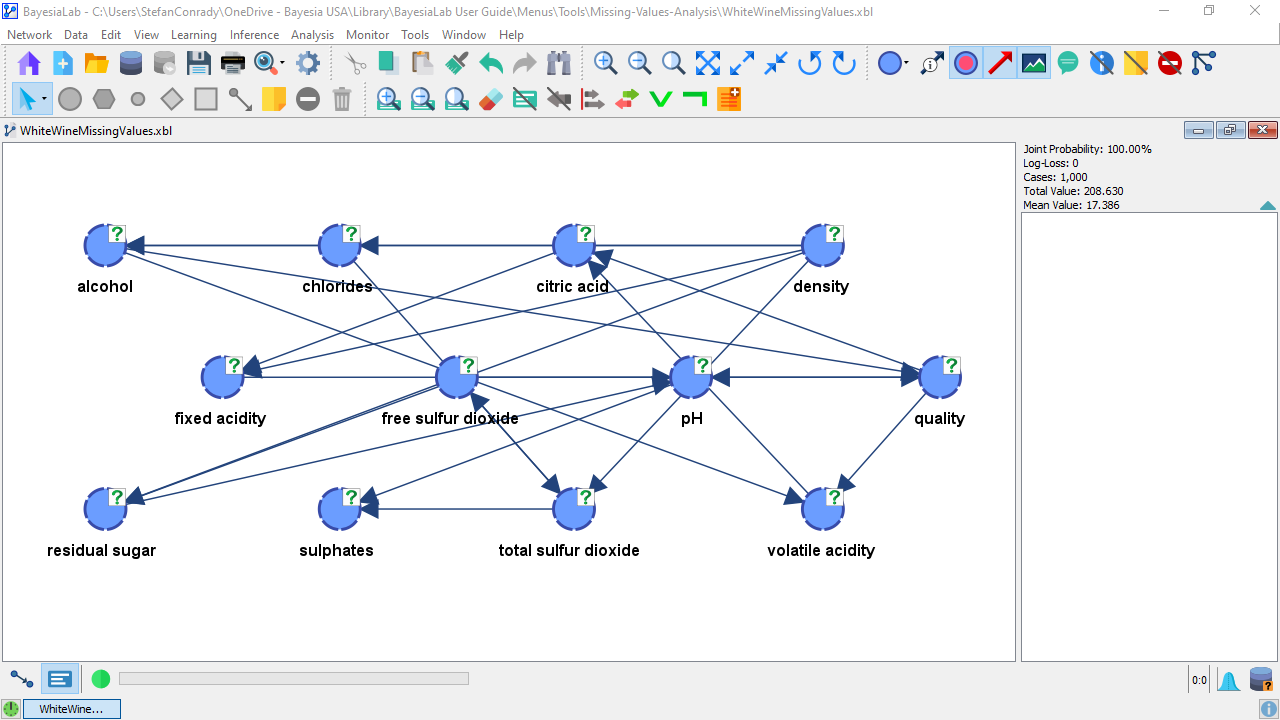
• Select Main Menu > Tools > Missing Values Analysis.

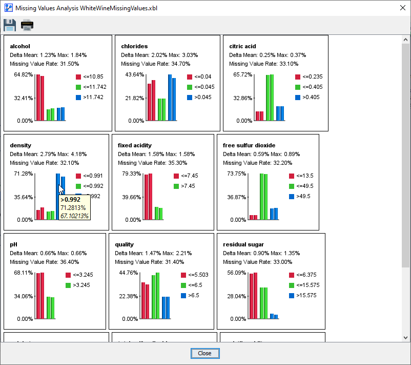
• In this window, bar charts for each node show the impact of using BayesiaLab's network-based Missing Values Processing:
  • Each panel represents the distributions of a node, sorted alphabetically by default.
  • Within each panel, pairs of color-coded bars represent the probabilities of the corresponding states. Each state has a distinct color within a panel.
  • Within each pair of bars:
    • The left bar represents the estimated probability of the state with Missing Values Processing given an unconnected network.
    • The right bar represents the estimated probability of the state computed using Missing Values Processing based on the given network.
  • Hovering over a set of bars shows a Tooltip with the numerical values of the state's probabilities.
  • For example, in the screenshot, PUnconnected(density > 0.992) = 71.2813% and PNetwork(density > 0.992) = 67.10213%. Using the network-based Missing Values Processing, the probability of the top state of the node density is lower by approximately 4 percentage points.
  • Several statistics are reported across the top of the panel:
    • Delta Mean: The difference in the mean value of the distribution due to network-based Missing Values Processing.
    • Max: The maximum delta in the probabilities among the states of the node represented by the panel.
    • Missing Value Rate: The percentage of missing values for the variable in the corresponding dataset.
  • By right-clicking on the background of the report window, you can change the appearance of the panels:
    • Sort Monitors:
      • Default Order: Panels sorted in the original order of variables in the dataset.
      • Names: Panels sorted alphabetically by node names.
      • Mean Delta: Panels sorted by delta in mean values, from high to low.
      • Max Delta: Panels sorted by the maximum delta in node state probabilities.
      • Missing Value Rate: Panels sorted by the proportion of missing values, from high to low.
    • Sort States:
      • Default Order: Keeps states in their original order.
      • Increasing Delta: Reorders states within each node to show the smallest delta first.
      • Decreasing Delta: Reorders states within each node to show the largest delta first.
      • This is helpful for nodes with strictly categorical states that do not have an implicit order.
  • You can also change how the content of each panel is displayed:
    • Relative Scale (default): The bar with the highest probability within a node defines the maximum y-axis value; the smallest defines the minimum. This prevents visual comparison across panels since each has its own scale.
    • Show Long Names: Activates the display of long names for nodes.
    • Show State's Long Names: Activates the display of long names for states.

Workflow Illustration