Target Precision

Context

• The Target Precision is one of the measures that can be computed in the Structural Coefficient Analysis and plotted in the Curve window.
• When plotted, the Target Precision can help you determine an appropriate value for the Structural Coefficient given your dataset and the learning algorithm you selected.
• The Target Precision metric is intended to be used primarily in the context of Supervised Learning.

Usage

• To illustrate the Target Precision metric, we use a sample network that predicts contraceptive use of married Indonesian women as a function of demographic attributes. This model is based on a subset of variables from the 1987 National Indonesia Contraceptive Prevalence Survey, which is available from the UCI Machine Learning Repository (opens in a new tab).

NICPS.xbl

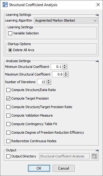
• Now, we perform a Structural Coefficient Analysis: Main Menu > Tools > Multi-Run > Structural Coefficient Analysis.
• We follow the overall workflow introduced in Structural Coefficient Analysis.
• Given that this is a predictive model, we select a  Supervised Learning algorithm from the settings window.
• More specifically, we choose the Augmented Markov Blanket and examine a range of 0.05 and 0.5 for the Structural Coefficient in 10 iterations.
• In the context of a predictive model, the Target Precision is one of the key metrics to evaluate.
  
• The dataset associated with this model is split into a Learning Set and a Test Set, as indicated by the  symbol tagged onto the database icon  in the lower right-hand corner of the Graph Window.
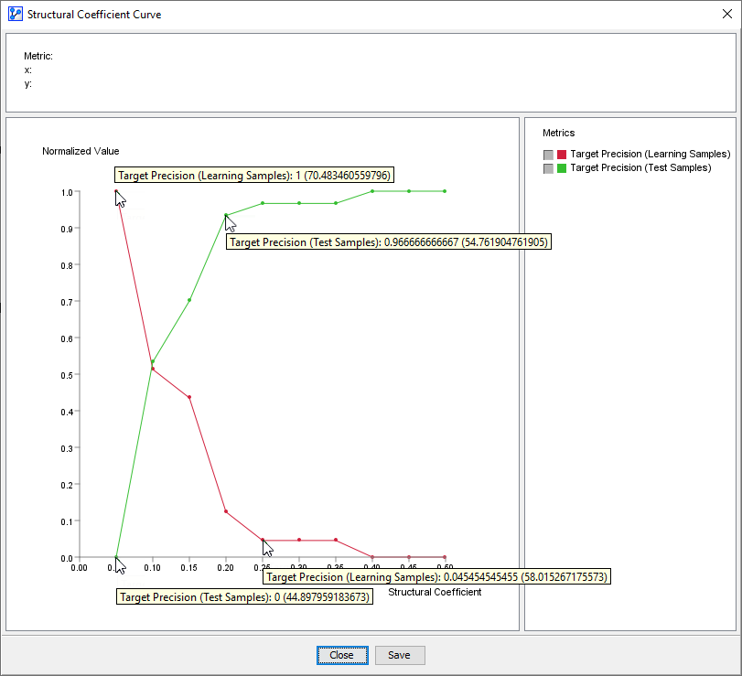
• Given the split, the Structural Coefficient Analysis calculates the Target Precision separately for the Learning Set and the Test Set.
  
• Note that the y-axis is normalized, but you can view the absolute values by hovering over individual points. The values in parentheses are the non-normalized values of Target Precision.
• In general, reducing the Structural Coefficient (x-axis) increases the Target Precision (y-axis) for the Learning Samples (red curve).
• Hence, it is always tempting to decrease the Structural Coefficient in pursuit of higher predictive performance.
• And, for SC>0.25, Target Precision (Learning Samples) appears relatively flat.
• For , the Target Precision (Learning Samples) increases very rapidly, potentially suggesting a good predictive performance. However, the performance of the model with regard to the learning set is of little value if it doesn't hold up in out-of-sample testing.
• And, indeed, the performance for does not hold up for the Test Set (green curve).
• While, for SC>0.25, Target Precision (Test Samples) appears flat, too, for , Target Precision (Test Samples) decreases very rapidly.
• In absolute terms, at SC=0.05, the Target Precision (Learning Samples) of 70% is vastly different than the Target Precision (Test Samples) of 45%. This is a very clear sign of overfitting.
• So, learning with an extremely low value of SC=0.05 would clearly lead to a model that cannot generalize beyond the learning sample.
• As a result, we can use the two curves as an additional visual guide for staying clear of potential overfitting.
• Note that this is not a hard-and-fast rule. Rather, you should use this Target Precision plot in the context of all the other available plots.