Chapter 12: Attribution, Contribution, and Counterfactuals

1. Attribution, Contribution, and Counterfactuals

   Attribution and contribution often appear in a similar context and are both concepts that are closely related to causality. In general, attribution identifies a source or cause of something observed. In marketing, attribution has a somewhat special meaning and often refers to the origin of a consumers’ journey towards an outcome. Thus, observed outcomes are attributed to specific prior touchpoints, such as website visits or a ad clicks (Julian, 2013). Conversely, events of that kind can be considered “drivers” of outcomes.

   Contribution has been proposed as a broader concept that involves a broader range of marketing drivers, on- and offline, and how they lead to a desired outcome (ibid.). As such, contribution is certainly a causal concept, too. The amount of contribution represents the degree of influence of one driver and compares it to any other drivers.1

   Definition of Contribution

   Despite its intuitive appeal, contribution is an elusive concept that lacks a formal definition in the sciences, in general, and in marketing, in particular. To operationalize contribution, we propose to distinguish between two types, which we shall call Type  1 and Type 2 Contribution.2 Both types rely on computing the difference between factual and counterfactual outcomes corresponding to factual and counterfactual conditions of drivers.

   A factual outcome is simply an actual observation of a target variable. Associated with a factual outcome are drivers at their observed, factual levels. A counterfactual outcome is the result of drivers being set to hypothetical, counterfactual conditions. This begs the question how we can determine the counterfactual outcome. We must infer it, of course, with a causal model or, alternatively, with a model that facilitates causal inference, such a statistical model with confounders selected. The latter we just utilized for marketing mix optimization.

   A New Example

   The definition of Contribution and its calculation is ultimately very simple, even though its description turns out to be rather verbose. To keep our explanation and notation manageable, we briefly digress from the marketing mix example and introduce a much simpler domain as an example. A key reason for its simplicity is that we make up the new example purely for our convenience. As creators, we define the “laws of nature” as we like. Thus, we automatically have perfect knowledge of them.

   Knowing the ground truth in advance, we will more easily recognize what is happening in each step of the definition of Contribution and the calculation of related measures.

   Causal Driver Model

   The domain of our example consists of three independent drivers X1, X2, and X3 and one outcome Y. More specifically, we also know the data-generating process that produces the values of Y:

2. The straightforward nature of this function will help us to develop an intuition of how calculating the Contribution characterizes the “contributory” roles of X1, X2, and X3 in this function. For the same reason, we choose convenient value ranges for the drivers, i.e. X1, X2 ! [1,10] and X3 ! [1,15]. Finally, all drivers have a uniform distribution. On this basis we produce artificial 5,000 samples.

   Creating a Model from Data

   With our domain now manifested in data, we can switch viewpoints and look at the newly-produced data from an outsider’s perspective. The new objective is to recover the characteristics of this domain from the available data. While we now go through the motions of discovering the structure from data, we obviously have the advantage of knowing the ground truth already.

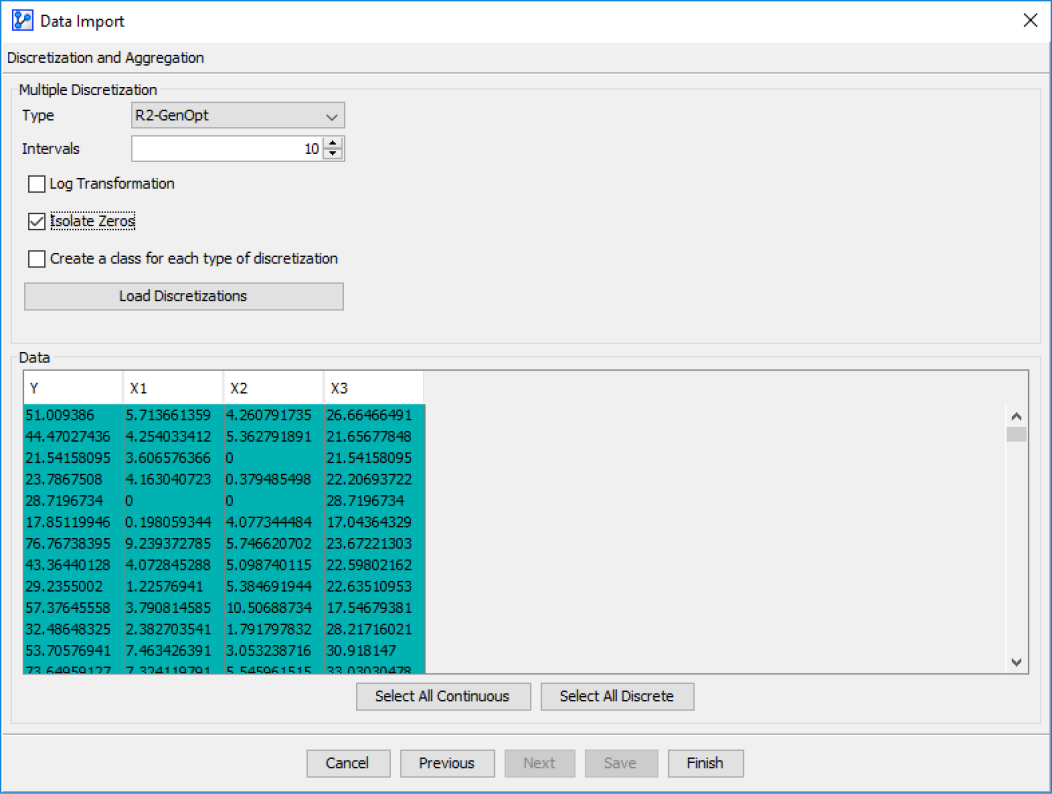
   We import the generated dataset into BayesiaLab, and go through the steps of the Data Import Wizard. Since we have already illustrated this process several times in earlier chapters, we omit most screenshots, only pointing out the Discretization step (Screenshot 12.147). Here we choose the R2GenOpt discretization algorithm with 10 intervals and select the Isolate Zeros option. The importance of this choice will become clear shortly, once we introduce the concept of Neutral State.

3. Data Import : Discretization

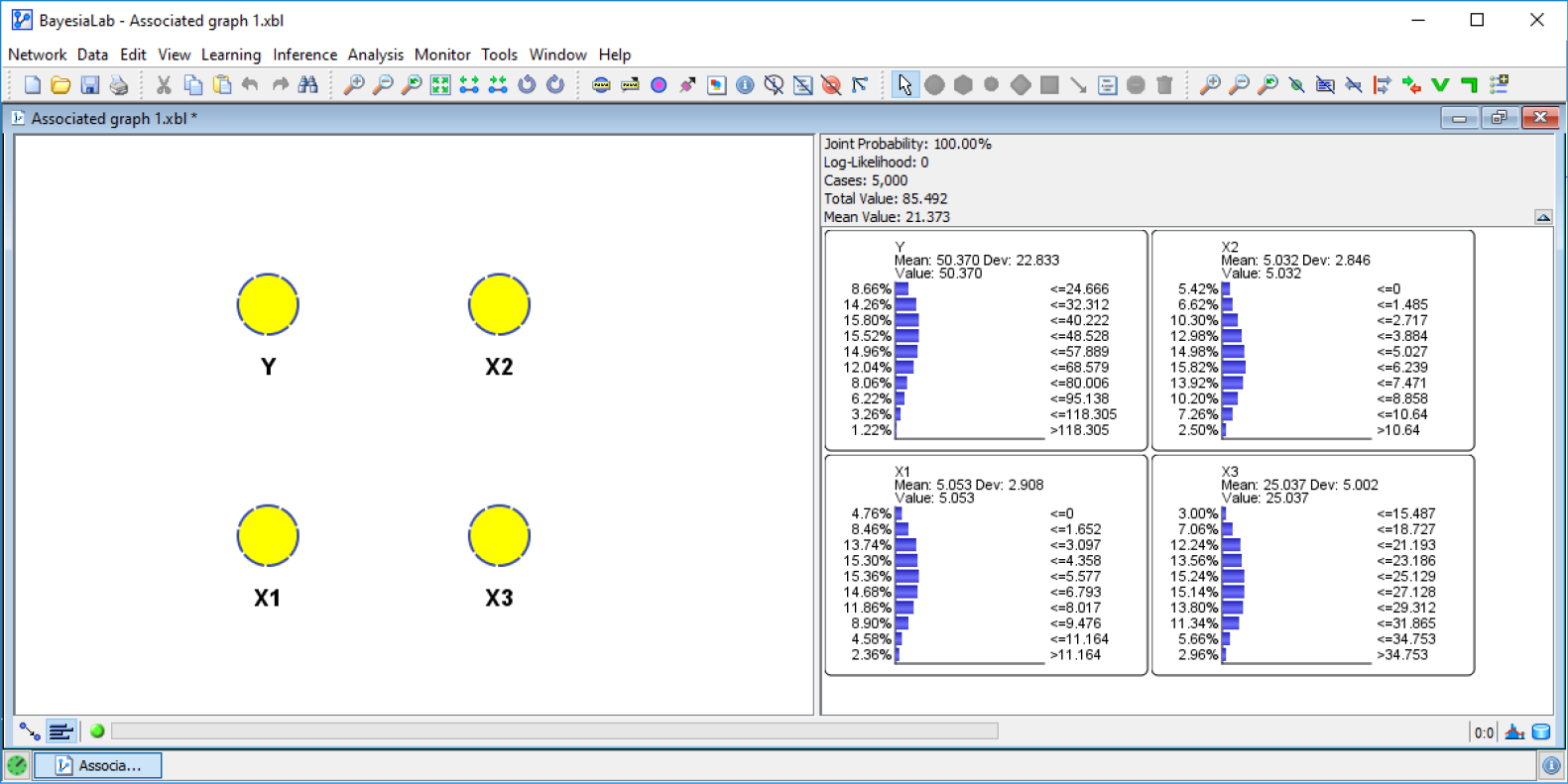
Upon import, we can see the distributions of the drivers.

1. Distributions of Imported Dataset

Next, we need to learn a structure. We designate Y as the Target Node and then run a Supervised Learning algorithm, such as the Markov Blanket algorithm. The result is Network 12.1, what appears to be a naive structure.

1. Learned Network Structure

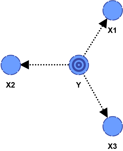
Clearly, this is network does not match the causal structure of the data-generating process. All arc directions are opposite to the true causal directions. This is one more example that shows that machine-learning algorithms, in general, cannot recover causal structures from data. Instead, BayesiaLab found a parsimonious approximation of the joint probability distribution of the underlying dataset.

Once again, this brings up the question of how to answer an inherently causal question, such as Contribution, with a non-causal model like this. In the previous chapter, we illustrated how the selection of Confounders suffices for the estimation of a causal effect. Here, we know that X1, X2, and X3 are Confounders. As a result, we can perform causal inference with Direct Effects on the basis of this machine-learned, non-causal model. As such, it will serve as the inference engine that we require to calculate Contributions.

Neutral State

We have already stated that computing Contributions will require us to compare outcomes as a function of factual and counterfactual conditions of driver variables. But what counterfactual conditions? The space of possible counterfactuals is infinite; it includes all states (or distributions) of drivers other than what we actually observed. So, which of these counterfactuals do we need for calculating Contributions? A particularly important counterfactual in this regard is the state of a driver that would have naturally occurred, had it not been for the state to which the driver was actually set.

For instance, when we speculate, “had it not been for X...”, we typically have a specific counterfactual in mind. When we say, “had it not been for the rain, I would gone to the park”, the implicit counterfactual is “no rain.” However, “snowstorm,” would also be a counterfactual, even though it is not the counterfactual we had meant when we said “had it not been for the rain...” So, in our everyday conversation we generally do not have to spell out counterfactuals. Rather, the context typically provides the most probable counterfactual.

However, if we wish to use a computer for reasoning, we do need to be explicit. This is why we introduce the concept of a Neutral State. It allows us to formally declare the intended counterfactual. In BayesiaLab, we use the Reference State to encode the Neutral State for each driver variable. This setting is available in the Node Editor under the Reference State tab. If we do not specify a Reference State, BayesiaLab uses the state with the smallest numerical value as the Neutral State for computing Contributions.

Type 1 Contribution

Now we have all the pieces in place to explain Type 1 and Type 2 Contributions. Type 1 Contribution is the difference between the actual outcome, which was observed with the driver at its factual state, and the hypothetical outcome, had the driver not been at the factual state but rather set to its counterfactual Neutral State. Needless to say, we only see the results of what we did and not of what did not do. This is why we need a causal inference engine, such as a full causal model or, alternatively, the machine-learned Bayesian network plus correctly specified Confounders. It allows us to infer the outcome as result of setting a driver to its counterfactual Neutral State.

Type 1 Model-Based Counterfactual Simulation

As it turns out, we can compute the outcome as a function of the Neutral State of a driver in two distinct ways: The first involves setting the driver to the Neutral State in our machine-learned model (Network 12.1). For instance, we compare Y at the factual distributions of all drivers (left set of Monitors in Screenshot 12.149) to the alternative scenario with X1 set to the Neutral State, while maintaining the factual, marginal distribution of the drivers X2, X3 through Likelihood Matching (right set of Monitors). Here, we use the default Neutral State of X1, which means xn=0.

1. Type 1 Model-Based Counterfactual Simulation

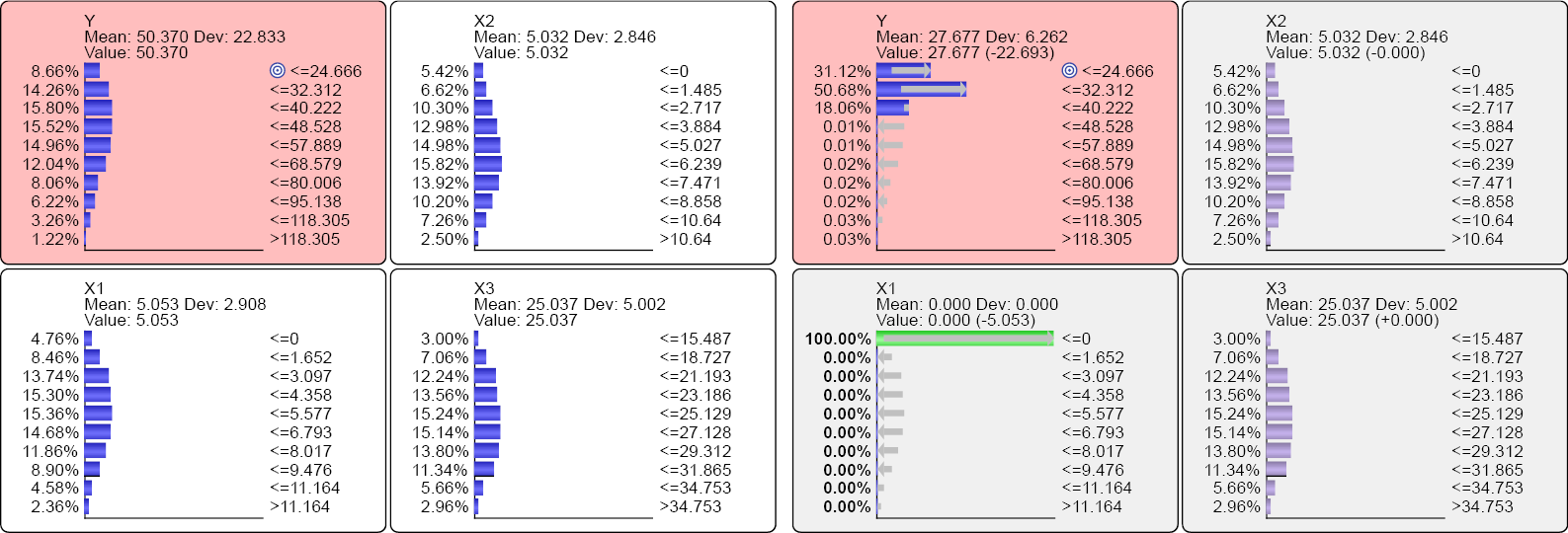
We can now compute the Type 1 Decomposition of X1 on this basis. It’s the difference between the expected values of Y in the left and the right panels. We speak of “decomposition” as we are decomposing Y into the components produced by the individual drivers.

Notation

For computing Decompositions and Contributions, we will need to go through large number of permutations of factual and counterfactual states and distributions, just like the above. Hence, we need to introduce a more precise way of referring to the conditions we are comparing. For the Type 1 Decomposition of X1, we can formally write.

1. In words, if we set X1 to the counterfactual, Neutral State (X1=0), the expected value of Y is reduced by 22.693. Conversely, setting X1 to the factual distribution, instead of the counterfactual Neutral State, adds 22.693 to the expected value of Y. With that, we can compute the Contribution C(X1):

2. Type 1 Data-Based Counterfactual Simulation

   The second approach is to perform inference at the record level of the underlying dataset. This terminology can be confusing. Even though we distinguish between “model-based” and “data-based” Contributions, calculating the data-based Contribution still utilizes the same model, i.e. Network 12.1. However, inference is performed at the record level, not at the aggregate level.

   We start with the original observations of the drivers and infer values of Y using Network 12.1. A small portion of this dataset is shown in Table 11.1. The observation number is denoted by i.

3. 

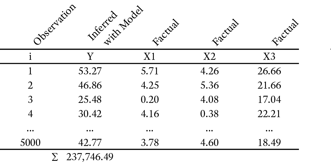
   From all inferred values Yi we compute the sum:

4. Next, we infer values of Y again, but this time with X1 set to the counterfactual Neutral State, X1=0, while keeping the observations of the other drivers unchanged at their original, factual values (Table 11.2).

5. 

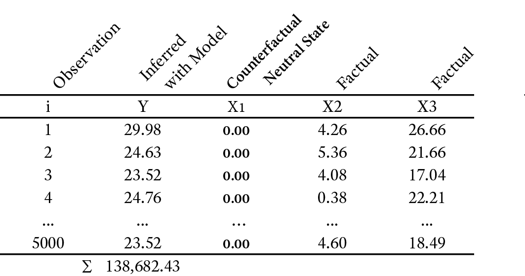
6. On that basis, we can compute a “data-based” Decomposition with regard to X1.

7. Note that the numerical value of the data-based Decomposition depends on the total number of observations i. We can now compute the Contribution CType1,Data(X1):

8. Type 2 Contribution

   Now we change the perspective. Instead of looking at the impact of the absence of X1, we now consider X1 to be the only available driver. This means we set the drivers X2 and X3, to their respective counterfactual, Neutral States and then compare the outcome Y for the factual distribution of X1 versus the outcome Y for the counterfactual Neutral State of X1. In other words, we consider X1 being the only driving force in the domain.

   Type 2 Model-Based Counterfactual Simulation

   Trying this out will make things clearer. In the left panels of Screenshot 12.150, we see X1, X2, and X3 set to their counterfactual, Neutral States. In the right panels, we see the Neutral State of X1 removed, thus allowing it to revert to its factual, marginal distribution. Note that for X1, X2 the Neutral State is 0. For X3, the Neutral State is X3≤15.487.

9. Type 2 Model-Based Counterfactual Simulation

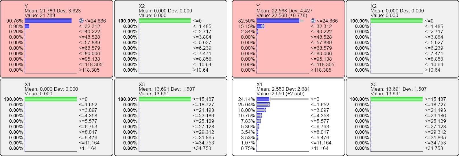
With these results, we can compute the Type 2 Decomposition DCType2,Model(X1):

1. In words, if remove Neutral State from X1 and allow it to return to the factual distribution, the expected value of Y increases by 2.550. With that, we can compute the Type 2 Contribution CType 2,Model(X1):

2. Type 2 Data-Based Counterfactual Simulation

   In the same way we performed a data-based counterfactual simulation to compute the Type 1 Decomposition and Contribution, we can do it for Type 2. This means that for every record in the dataset, we replace the observed, factual levels of X1, X2, and X3 with the counterfactual Neutral States and infer the values for Y. Then, we recompute all values of Yi by setting X1 to the observed, factual states in each record (Table 12.9)

3. 

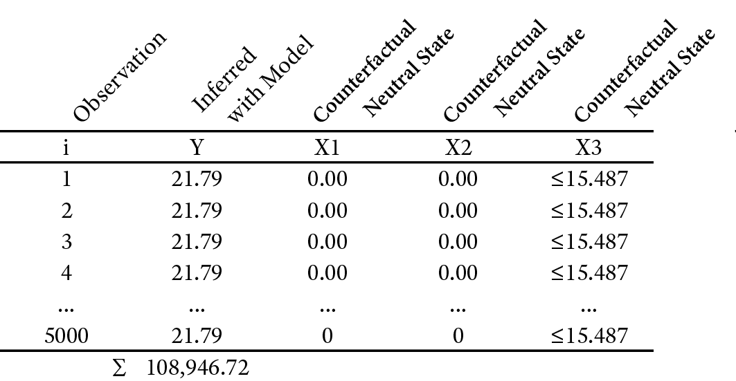
   Again, we compute the sum of all Y values.

4. Then, we set X1 to the observed, factual states in each record (Table 12.10).

5. 

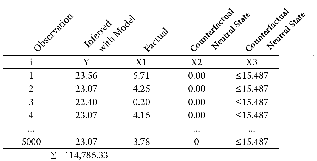
   Again, we compute the sum of all Y values.

6. This allows us to compute the Type 2 Decomposition DCType2,Data(X1).

7. Note that this data-based Decomposition once again depends on the number of observations i. The Type 2 Contribution is defined analogously to Type 1.

8. Computing the Baseline Contribution

   When we introduced the concept of contribution, we briefly mentioned that a baseline component can also contribute to the outcome variable in a domain. We often encounter this concept when we speak of “baseline sales,” which we think of as the natural demand that exists with minimal or zero promotional effort. The idea of a certain base-level outcome with zero input can be nicely implemented in regressions. We typically interpret the y-intercept as “baseline,” i.e. the y-value given that x equals zero. How can we translate this concept into our nonparametric approach?

   As it turns out, the way we compute the baseline contribution is similar to setting x to zero in a regression. In our example, we will set X1, X2, and X3 to their respective counterfactual, Neutral States and then infer the expected value of Y. Once again, we do this first on the basis of the model (Network 12.1) and then with the dataset.

   Model-Based Baseline Contribution

   In Screenshot 12.151, the left set of Monitors show the marginal distributions of all variables.

9. 

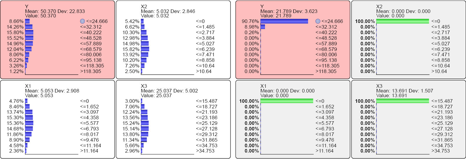
   This gives us the expected value of Y, which we will subsequently use in the calculation of the Contribution.

10. In the right set of Monitors, X1, X2, and X3 are set to the their respective Neutral States. The expected value of Y provides the Baseline Decomposition, DC(Y). This is the expected value of Y given that all drivers are set to their Neutral States.

11. With that, we can compute the Base Contribution CModel(Y):

12. In other words, 43.3% of the mean value of Y exists with all drivers to their Neutral States. Thus, we can say that 43.4% of the value of the outcome variable comes from a baseline component.

    Data-Based Baseline Contribution

    We repeat the same calculation using the dataset. We define the Baseline Decomposition of Y as the sum of Yi, given that all drivers are set to their Neutral States. As it turns out, we have already generated the necessary table, i.e. Table 12.9.

13. Note that this data-based Decomposition once again depends on the number of observations. Now we divide DCData(Y) by the sum of the factual values Y to obtain the Base Contribution CData(Y).

14. Mean Contribution

    By now, we have computed the Contribution of the variable X1 in four different ways, i.e. CType 1, Model(X1), CType 1, Data(X1), CType 2, Model(X1), and CType 2, Data(X1). And, we have obtained four different values of Contribution. What does it mean that Type 1 and Type  2 Contributions have such different levels? Depending on the nature of the data-generating process that determines the values of the Target Node, neither Type 1 nor Type 2 may represent the correct contribution. Empirical assessments of known data-generating processes for the Target Node have shown that Type 1 and Type 2 Contributions either underestimate/overestimate or overestimate/underestimate Contributions. As we know that data-generating process of our example is nonlinear, we can easily understand that a single measure cannot possibly capture Contribution. So, what is the most appropriate Contribution that we should use for interpretation?

    We propose to utilize the Mean Contribution. It can be calculated on the basis of the Model (12.19) or the dataset (12.20).

16. Now that we have computed the mean Contributions of X1, we need to repeat the same process for X2, and X3.

    Normalization

    Once we have calculated the Mean Contributions of all drivers, plus the Base Contribution, we apply normalization: If the sum of the Mean Contributions of all drivers and the Base Contribution is greater than 1, we normalize the Mean Contributions to obtain a sum of 1. If the sum is smaller than 1, the balance is added to the Base Contribution.

    Final Contribution

    By now we computed a four contribution measures for each driver variable, plus two types of base contributions. We may feel that we are no longer able to see the forest for all the trees. It is all coming together in what we call the Final Contributions, which is the average of the normalized mean Contributions.

17. After computing the sum of all Final Contributions, the Final Base Contribution is defined as:

18. The above series of calculations highlights how much effort is required to quantify contribution in a meaningful way, even though contribution as a concept appears intuitive.

    Contribution Analysis in Practice

    In BayesiaLab, all of the calculations for Decomposition, Base Contribution, and variable-specific Contribution are combined and automated in the Contribution Analysis function. We can launch it via Analysis > Report > Target Analysis > Contribution Analysis.

19. Type 2 Model-Based Counterfactual Simulation

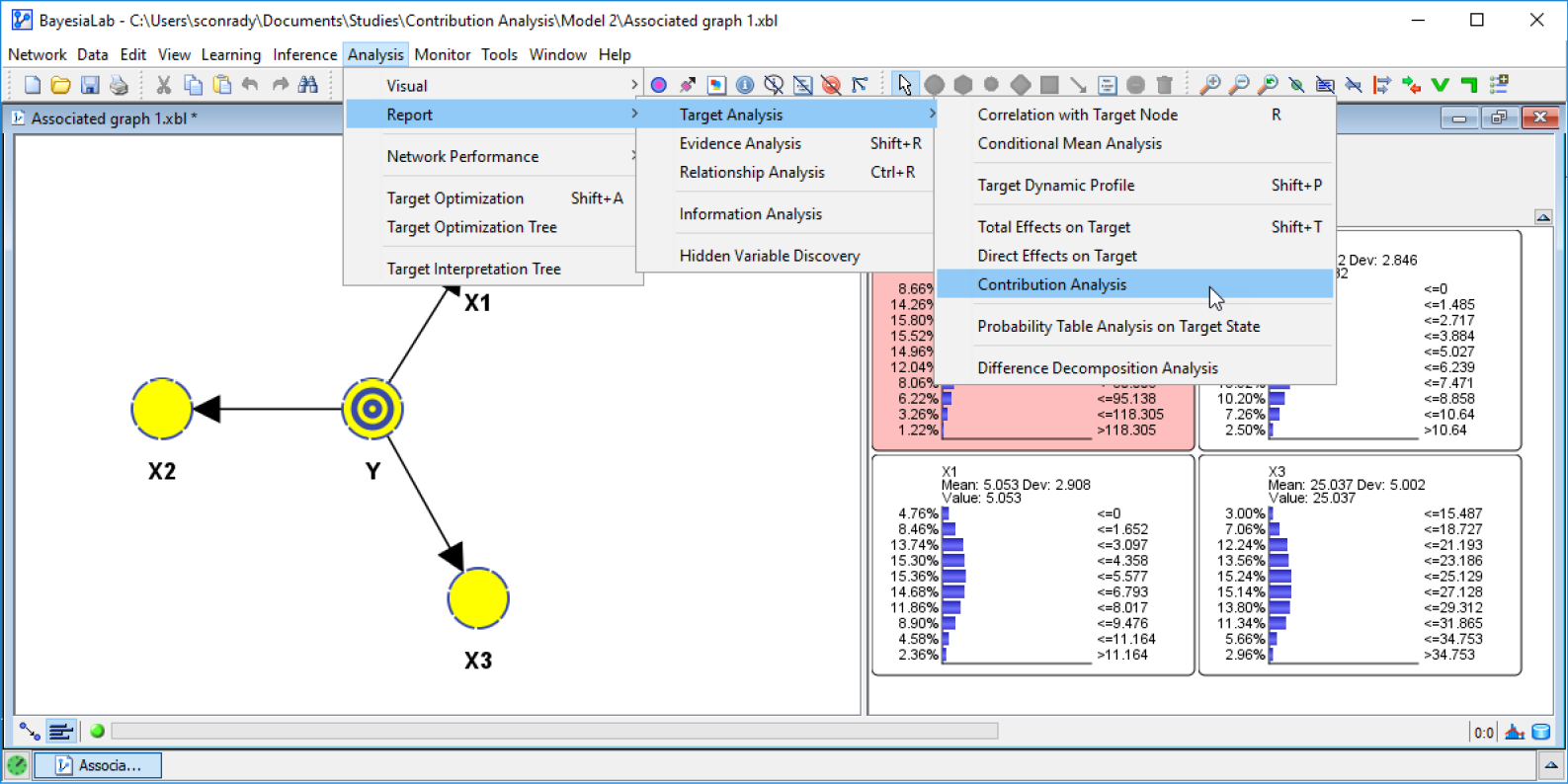
BayesiaLab prompts us to select the node for which the analysis should be performed. Furthermore, we can optionally specify the Output File for saving the Decompositions and Contributions for every single observation in the dataset (Screenshot 12.153).

1. Contribution Analysis

The output is in CSV format and contains:

• Normalized Base Contributions and Mean Contributions
• Type 1 Normalized Decompositions and Contributions
• Type 2 Normalized Decompositions and Contributions

1. Contribution Analysis Report

Now we have a very comprehensive generalization of how the values of a Target Node decompose into contributions coming from each driver. Put differently, we can now attribute an observed outcome to individual drivers.

Curves

The Curves function is a visualization the output file. We can use it to assess contributions record by record. Typically, this is of interest with time series data and can show how Contributions evolve over time. Screenshot 12.155 shows the last 18 records of the dataset of this example. The intervals on the x-axis correspond to the sequence of observations in the dataset. The y-axis represents the value of the Target Node.

2. Contribution Plot Produced by the Curves Function

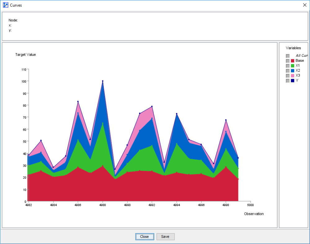
This plot layers the contributions so that we can see how the final value is composed. The bottom layer represents the Base Contribution, followed by the Contribution of each driver.

Synergies

The term “synergy” has been a buzzword in business management for a long time. It refers to the benefit of joining forces. This can involve companies, resources, or individuals working together. In that sense, synergy is very close in meaning to the Greek word from which it derives, συνεργός (synergos), which translates into co-worker or fellow worker. When we speak of the benefits of synergy, we typically mean that a combined effort produces an effect that is greater than what would be the sum of the effects from separate efforts. This is expressed in the popular quote, “the whole is greater than the sum of its parts,” which has been informally attributed to the philosopher Aristotle.

This is precisely what we try to quantify in the Synergies section of the Contribution Analysis Report. Here, BayesiaLab compares the joint contributions of two drivers to the sum of their individual contributions. Once again, we compute this measure on the basis of the model and the database, using the following, Type 2 counterfactual question:

What is the mean value of the Target Node, if the pair of drivers under study are kept at their original marginal probability distributions while all Confounders are set to their Neutral States?

Model-Based Synergy Decomposition

3. Model-Based Synergy

4. Data-Based Synergy Decomposition

   In parallel to the earlier calculations for Contribution, we compute Synergy also with the dataset. We ask the question, “what is the value of the Target Node for each observation, if the pair of drivers under study are kept at their original values while all Confounders are set to their Neutral States?”

5. Data-Based Synergy

6. Mean Synergy

   Similarly to the Mean Contribution, we propose the Mean Synergy as a suitable measure to characterize the synergy benefit of a pair of variables:

7. Now that we know how Synergies are computed in BayesiaLab, we return to the Synergy section of the Contribution Analysis Report (Screenshot 12.156).

8. Synergies

The Mean Synergy of the node pair X1 and X2 stands out as particularly strong. This should not be a surprise given the data-generating function we had originally specified (12.28). We intentionally built the synergy between X1 and X2 into the data-generating process:

9. However, the point of this exercise was that we can recover synergies from an underlying dataset with the help of a machine-learned model and assumptions regarding the Confounders. In the same way we can estimate causal effects without the full causal understanding of the domain, we can calculate Contributions.

   Also, BayesiaLab only computes Synergies for pairs of drivers. Obviously, there exist Synergies between any number of drivers. In fact, for larger models, there could be an astronomical number of driver combinations to evaluate. However, skipping the evaluation of all of them is not necessarily an omission.

   By virtue of utilizing a Bayesian network model, we are implicitly accounting for all synergies between variables during effect analysis and optimization. This means, we automatically include synergistic effects, even though we may not have identified them. Furthermore, as we perform effect analysis or optimization, there could be synergy effects between any number of variables beyond pairwise effects.

   Marketing Mix Model

   This brings us back to our marketing mix example from the previous chapter. We now have the ability to see what each marketing channel is contributing towards Sales.

10. Contribution Analysis Report

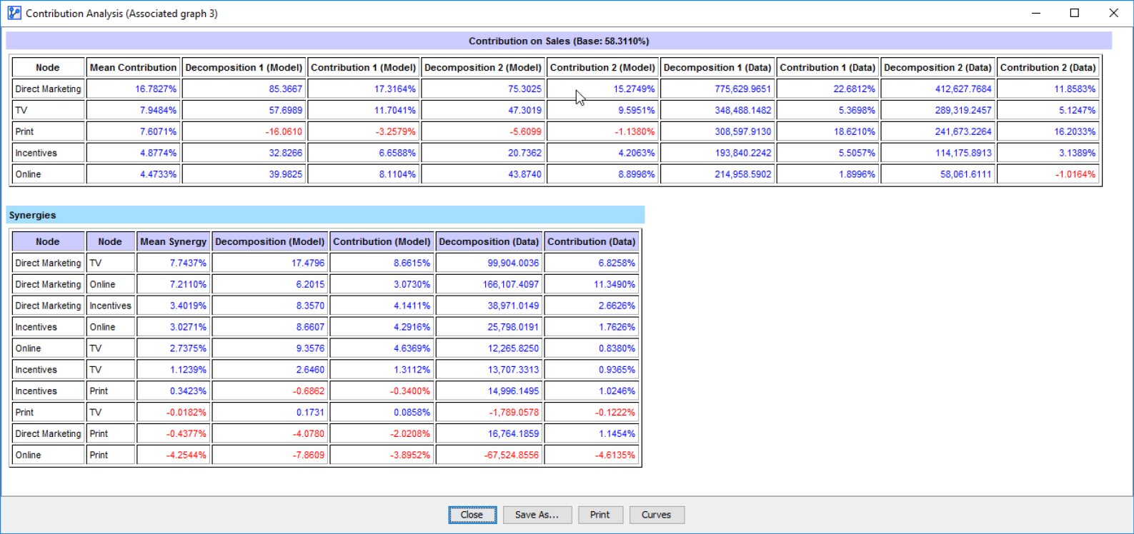
These results also show that Contributions and Synergies can be negative. A negative contribution suggests that a driver at the observed levels resulted in a lower values of Sales compared to what would have been the case if the driver had been observed at the Neutral State. In the context of ice cream sales, for instance, if the temperature over the observed time frame was below the Neutral State, the Contribution would be negative, even though an increase in temperature has a positive effect on ice cream sales.

Negative synergies imply that the joint application of to driver variables produces something less than the sum of the individual drivers. Practically speaking, this could mean that drivers are at least partially redundant. For example, a consumer who has already been persuaded through one marketing channel is exposed again through another one. However, this is not to be confused with a negative Direct Effect.

Conclusion

It is worth noting in conclusion how seemingly obvious concepts like contribution and synergy require a disciplined theoretical framework, plus a substantial computational effort, to deliver values that are consistent with our intuition. In particular, we require a model the facilitates causal inference, and we need a formal definition of counterfactuals for the domain under study. This is a rather tall order indeed, which stands in contrast to the simplicity of the percentage values that are produced. As such, context plus caveats are mandatory for communicating Contributions and Synergies.

1. Contribution Analysis Output File

This gives us a sense what each driver contributed towards the Target Node’s value in each observation. In addition to the detailed record-by-record output in the CSV file, we also receive a report that contains all Contribution types for each driver variable plus the Base Contribution (Screenshot 12.154).

We always assert a causal meaning when we use the word “driver”, i.e. a driver is always a cause, similar in meaning to “treatment.” However, “driver” a is not reserved term in BayesiaLab.

From now on, when Contribution is capitalized and in bold type, we refer to the quantity computed as per the proposed definition. In lowercase, contribution is understood in the conventional sense.